Chapter 9 Stokes Flow
In this chapter, we will be considering situations where inertial forces are negligible such that the flows have small Reynolds numbers. Such flows are named Stokes flows after George G. Stokes who first calculated the drag on a sphere moving through a viscous fluid. The applications of Stokes flows are wide ranging, from biological applications at the small scale (e.g. the swimming of microorganisms) to geological applications at the large scale (e.g. the flow of lava).
9.1 Recap: Governing Equations
9.1.1 Navier-Stokes Equations
For an incompressible fluid, the equations for mass and momentum balance are (see §2.8 and §2.9):
| (9.1) |
where is the velocity, is the constant density, is time, is the stress tensor and is a body force (i.e. ).
Internal viscous stresses are produced by deformation. The fluid is Newtonian if the relationship between the rate of deformation () and the stress is local, linear, instantaneous and isotropic. If the fluid is also incompressible, the Newtonian constitutive law is
| (9.2) |
Substituting this into the momentum balance (9.1) gives the incompressible Navier-Stokes equations:
| (9.3) |
9.1.2 Reynolds number
To non-dimensionalise the problem we write
| (9.4) |
where is a characteristic velocity scale, is a characteristic lengthscale, and is a characteristic pressure scale. Substituting these into equation (9.3) when and rearranging we arrive at
| (9.5) |
where . We choose the viscous scaling for the pressure (we could have chosen the alternative inertial scaling ). This leaves one non-dimensional group called the Reynolds number:
| (9.6) |
where is the kinematic viscosity ( is denoted the dynamic viscosity). In this section we will be focusing on the limit where such that inertia is negligible and we can ignore the left-hand side of (9.5). The mass and momentum balance, known as Stokes Equations, are then given by
| (9.7) |
9.1.3 Energy and Dissipation
Taking the dot product of the full momentum equation (9.1) with the velocity and integrating over a volume gives
| (9.8) |
This can also be written in summation convention
| (9.9) |
Rearranging, applying the divergence theorem and mass conservation, the left-hand side becomes
Similarly, the right-hand side becomes
The mechanical energy equation is then written as
| (9.10) |
where
-
1.
the rate of change of kinetic energy in volume is due to:
-
2.
the flux of kinetic energy over the boundary ,
-
3.
the rate of working by body forces in volume ,
-
4.
the rate of working of surface forces in ,
-
5.
and the stress working in volume .
The mechanical energy equation above is for a general continuum. We can now look more specifically for a Newtonian viscous fluid with constitutive law,
| (9.11) |
The stress working per unit volume then becomes
| (9.12) |
Remembering some properties of the rate of strain and rotation tensors, we know that
| (9.13) |
| (9.14) |
Hence, the stress working, also known as the viscous dissipation , per unit volume is given by
| (9.15) |
The viscous dissipation describes the rate of loss of mechanical energy due to friction in the volume .
9.1.4 Additional comments
The approximation of Stokes Flow is good if the velocity or length scales are small (e.g. swimming microorganisms), or the dynamic viscosity is large (e.g. in geophysics, flow in porous media, or the flow of lava or ice). Some examples are:
| Sperm in water: | ||||||
|---|---|---|---|---|---|---|
| Mantle: |
(See E. M. Purcell (1977) Life at Low Reynolds Number, American Journal of Physics).
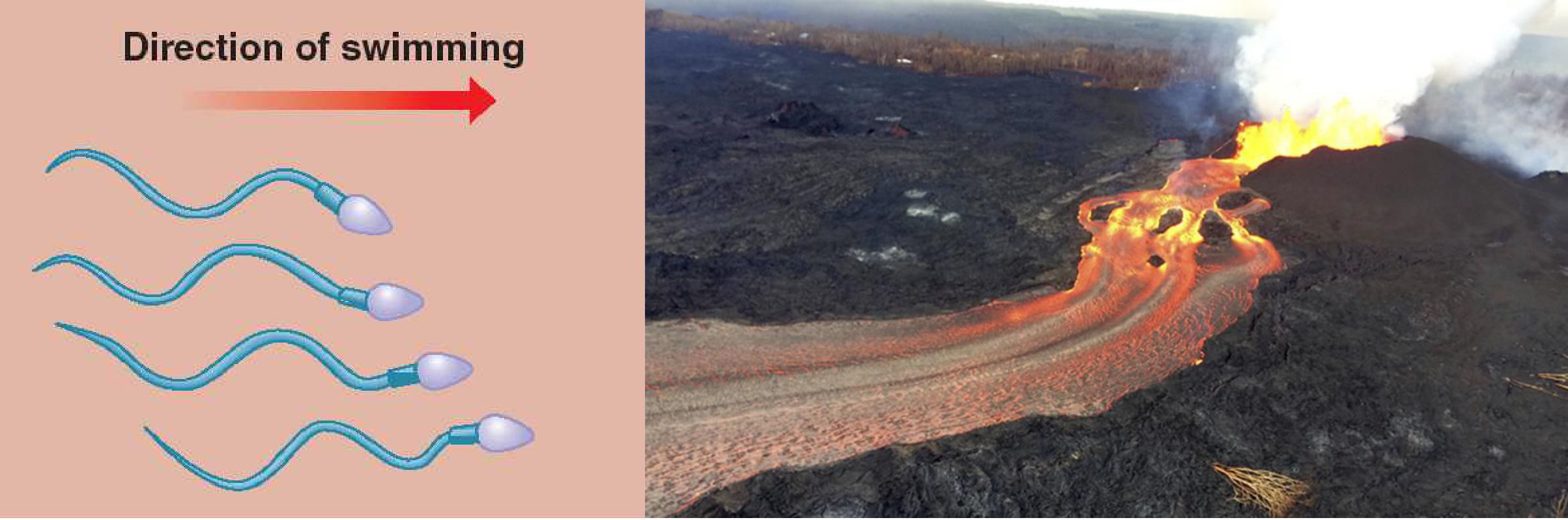
When approximating the Reynolds number, there are some caveats. Firstly there may be more than one relevant lengthscale, e.g in Lubrication theory later in the course the vertical lengthscale is much smaller than the horizontal lengthscale . These lengthscales may also vary with position e.g. flow past a body where in the far field where is the radial distance away from the body. Finally, the time scale may not be but instead may be specified by an external driving force e.g. an oscillating boundary condition with timescale .
9.2 Properties of Stokes Flows
-
1.
Instantaneity Instantaneity of the flow means there are no time derivatives , so no inertia. The flow has no memory and only knows about the current boundary conditions and applied forcing, responding immediately to any changes. The flow is said to be “quasi-steady” as can vary in time if the boundary conditions and applied forcing varies in time.
E.g. for a translating body with speed , the fluid force on the body is proportional to its velocity and not to its acceleration .
-
2.
Linearity: Linearity means that the flow is linearly forced whether it is by a boundary motion or body force. In Stokes Equations there is no , so and are linear in and the boundary conditions.
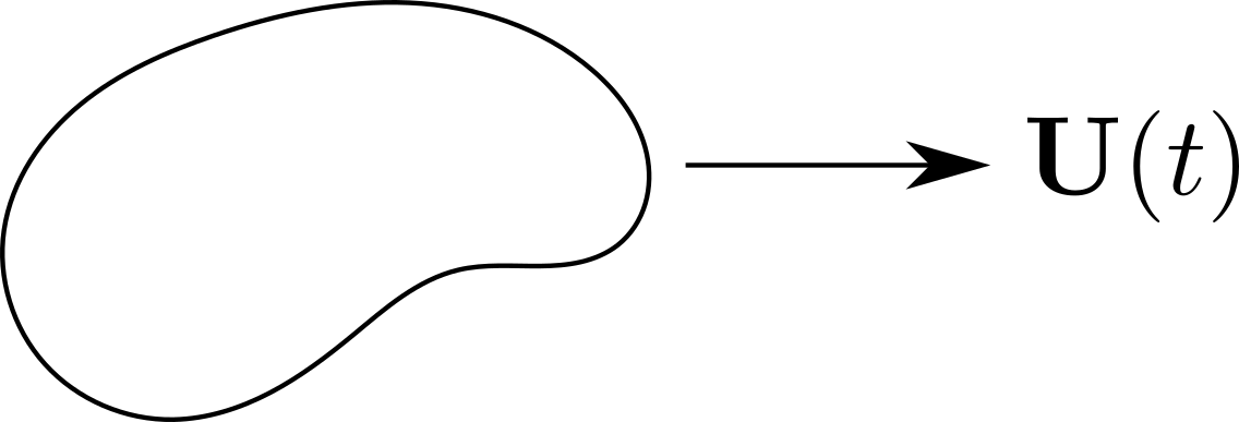
Figure 9.2: A translating body. -
3.
Reversiblity: Reversible in time: if you apply a force in and then reverse the force and its history in then the flow reverses and the fluid particles return to their starting position.
Reversible in space: reversibility in time and the symmetry of geometry can often be used to rule out some components of velocity .
E.g. does a sphere sedimenting next to a vertical wall migrate towards the wall?
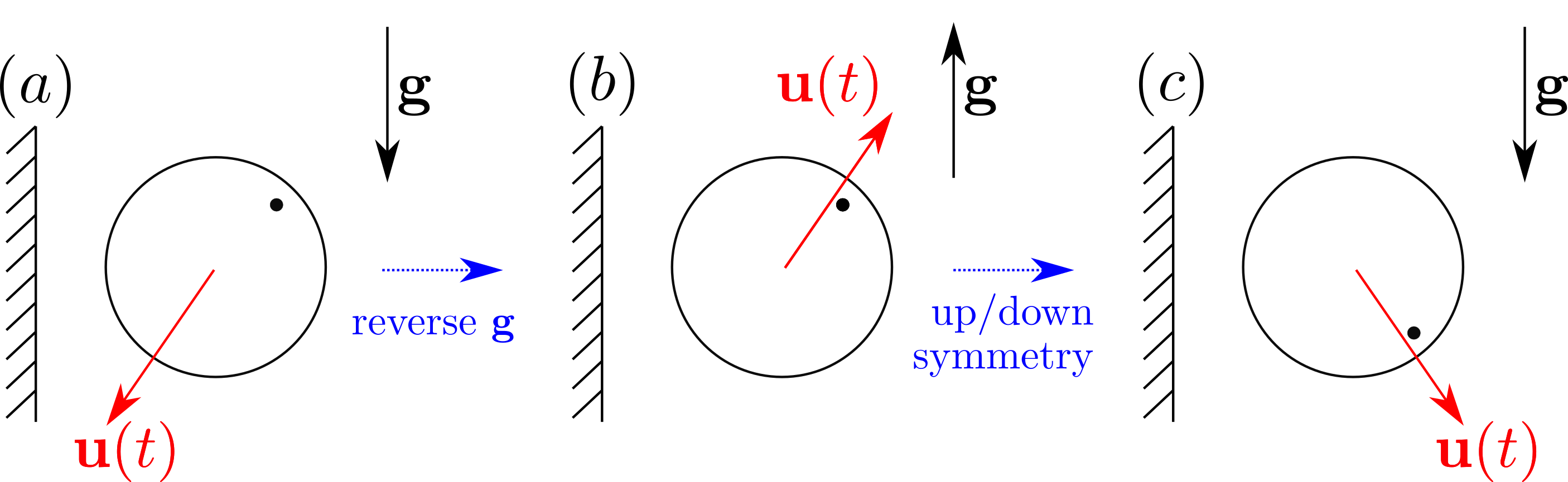
Figure 9.3: Sedimenting sphere. Reversing the forcing must reverse the velocity by reversibility in time. Because of the symmetry of the sedimenting sphere we can reverse the system in . In order for (a) to be the same as (c) we require the sphere to fall vertically with no horizontal component. -
4.
Forces Balance:
Since there is no inertia the forces in the system must balance:
(9.16) Applying the divergence theorem then gives
(9.17) This checks the consistency of the stress boundary conditions. In a similar way, we can check the consistency of the velocity boundary conditions by intergrating the mass balance equation:
(9.18) -
5.
Work Balances Dissipation: Since there is no kinetic energy in the mechanical energy balance, from (9.10) we know that the work done by body and surface forces must balance the viscous dissipation in a given volume:
(9.19)
Useful Lemma: Let be an incompressible flow and be a Stokes flow with body force such that
| (9.20) |
Then,
| (9.21) |
Proof: We know that for a Stokes flow Hence,
| (9.22) |
due to incompressibility. Also, using the fact that is symmetric and that where is antisymmetric, we find
| (9.23) | ||||
| (9.24) |
Integrating over a volume and applying the divergence theorem then gives the result:
| (9.25) |
-
6.
Uniqueness: Uniqueness means that each Stokes flow is unique but can be represented in many ways. Let and be Stokes flows with the same body forcing and boundary conditions, i.e. in and either or on . Then .
To show this we consider the flow . From the property of linearity we know that must also be a Stokes flow with and either or on . From the above lemma, we can show that
(9.26) The integrand is positive so must vanish, hence . The flow is strain less so must be in solid body motion . Velocity boundary conditions of on imply that everywhere. [N.B. Stress conditions can lead to solid body motion].
-
7.
Minimum Dissipation: Among all incompressible flows with the same velocity boundary conditions, the dissipation is minimised by the Stokes flow with no body force.
Let be an incompressible flow and be a Stokes flow with and . We know that
(9.27) (9.28) from the lemma above. Therefore the dissipation is minimised for a Stokes flow
(9.29) -
8.
Geometric bounding: The minimum dissipation theorem can be used to calculate bounds for the flow around more complicated geometries. Consider a cube of side length moving at a velocity in a fluid, with drag force , and Stokes flow outside the cube.
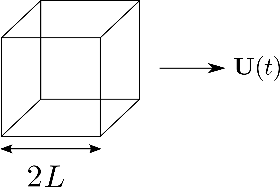
Figure 9.4: Stokes flow around a translating cube We can write down the dissipation (using the Stokes flow property that work balances dissipation) as
(9.30) We are considering the dissipation in the volume outside of the cube so the normal to the surface points inwards. This is the opposite to calculating drag on the sphere and hence a minus sign is introduced. Now consider a sphere that just contains the cube so have side length . We can define an incompressible flow outside the cube made up of a Stokes flow outside the sphere and a flow with constant flow velocity between the sphere and the cube:
(9.31) The dissipation for this flow is given by
(9.32) where we have used the fact that the strain rate for a flow with constant velocity is zero () and the drag on a sphere of radius is . Finally, we know that the dissipation is minimised for a Stokes flow, and hence
(9.33) This gives an upper bound on the drag force on the cube. We can go through a similar argument to find a lower bound by considering the flow outside of a sphere that just fits inside the cube, with radius . We won’t repeat the analysis here but the result should give
(9.34) -
9.
Reciprocal theorem: Consider Stokes flows and in a given volume with different boundary conditions and no body forces. Taking the first flow to be the Stokes flow , the second flow to be the incompressible flow and using the above we have
(9.35) If we instead take the second flow to be the Stokes flow , in a similar manner we have
(9.36) Equating the two we find that the rate of working of surface forces of flow 1 against flow 2 equals the rate of working of surface forces of flow 2 against flow 1 (reciprocal theorem):
(9.37) If the boundary conditions are a uniform translation velocity , the reciprocal theorem reduces to
(9.38) where are the corresponding surface forces.
9.3 Stokes Flow Solutions
9.3.1 Representation as Harmonic Functions
Consider Stokes equations with body force :
| (9.39) |
| (9.40) | ||||
| (9.41) | ||||
| (9.42) |
Hence, and are harmonic and is biharmonic.
9.3.2 Papkovich-Neuber Solutions
A method for finding the solution of Stokes flows comes from the Papkovich-Neuber representation. Suppose we can write the pressure . Then
| (9.43) |
Using the incompressibility condition, we have
| (9.44) |
We can check this last relation:
| (9.45) | ||||
| (9.46) |
Any Stokes flow with can be written in terms of a harmonic vector and a harmonic scalar :
| (9.47) |
9.3.3 Spherical Harmonic Solutions
Spherical harmonic functions are used for solutions involving points, spheres and cylinders that have no preferred direction or orientation. Let the radial coordinate . We can show that , except when :
| (9.48) | ||||
| (9.49) |
All other harmonic functions with and are made up of
| (9.50) |
Harmonic functions that are bounded at are made up of
| (9.51) |
These solutions only depend on and and have no preferred orientation. Some useful derivatives to remember are:
| (9.52) | ||||
| (9.53) | ||||
| (9.54) | ||||
| (9.55) |
Since we know that Stokes flows are linear in boundary conditions and forcing, we can form Papkovich-Neuber solutions by multiplying them by constant scalars, vectors, tensors, and forming dot-products, for example
| (9.56) |
9.3.4 Tensors and Pseudotensors
When building these solutions there are some properties it is useful to recall about tensors. An th-rank tensor is a set of objects that transform like a product of vectors. For example, if is an th-rank tensor, then
| (9.57) |
where is a transformation matrix. Symmetry properties are tensor invariant, so if is symmetric (antisymmetric) under an exchange of and then is also symmetric (antisymmetric) under an exchange of and . Examples of tensors in our problems would be
| (9.58) |
In contrast, pseudotensors, such as the Levi-Civita , change sign under transformation by reflections. Examples of pseudotensors we will come across are
| (9.59) |
If we want to find the velocity using the Papkovich-Neuber representation, then we want and to be tensors.
9.3.5 Point Force and Source Flow
Point force (Stokeslet): We want to find the velocity field for a point force. Consider the following:
| (9.60) | ||||
| (9.61) |
We know that
-
by linearity, the velocity field must be linear in the forcing
-
solution must decay in the far field
-
there is no preferred direction in the problem, can use spherical harmonics
-
the velocity field must be made up of tensors
Using this information, we can now try to build harmonic functions and using the solutions in (9.50)-(9.51). Let’s try the following ansatzes:
| (9.62) | ||||
| (9.63) | ||||
| (9.64) |
The first ansatz is the only one that decays in the far field and will not blow up at the origin. We proceed by substituting into the solution (9.47):
| (9.65) |
To fully specify the solution we need to find . Going back to the problem statement, we want the solution to satisfy
| (9.66) |
(this is built into the Papkovich-Neuber representation), and
| (9.67) |
On a sphere , , the normal velocity can be calculated
| (9.68) |
| (9.69) |
The normal stress can also be calculated, but requires a bit more algebra:
| (9.70) |
with
| (9.71) |
| (9.72) |
Here, we have noticed that the integral marked is an isotropic second rank tensor so must be . We can determine the constant of proportionality by calculating the trace, . Hence, . Notice that is independent of . If we had chosen one of the other harmonic solutions with higher powers of , they would be too singular to satisfy the force condition.
Source Flow (Point mass source): We want to find the velocity field for a point source in three-dimensions. Consider the following:
| (9.73) | ||||
| (9.74) |
Strictly speaking this flow is only incompressible for as volume is not conserved at but generated there instead.
We know that
-
by linearity, the velocity field must be linear in the source flux
-
solution must decay in the far field
-
there is no preferred direction in the problem, can use spherical harmonics
-
the velocity field must be made up of tensors
Let’s try harmonic function
| (9.75) |
In a similar manner to the point force, the other harmonic solutions with higher powers of would be too singular to satisfy the source condition. Substituting into the solution (9.47) we find:
| (9.76) |
To find , we use the source condition at :
| (9.77) |
Hence, . The velocity field then becomes which is independent of viscosity . This is the three-dimensional extension of the potential flow for a point source studied in §6.
9.3.6 Motion of a rigid particle
A sphere of radius translating with velocity and rotating with angular velocity moves with velocity
| (9.78) |
and exerts a force and couple on the fluid. The dissipation in the fluid due to the particle is (using work balances dissipation)
| (9.79) | ||||
| (9.80) | ||||
| (9.81) |
where the normal points out of the fluid into the body, with
| (9.82) |
exerted on the fluid by the sphere.
9.3.7 Translating Rigid Sphere
Velocity Field: We would like to calculate the velocity field for a rigid sphere of radius translating with velocity . Consider the following:
| (9.83) | |||
| (9.84) |
We know that
-
by linearity, the velocity field must be linear in the forcing
-
solution must decay in the far field
-
there is no preferred direction in the problem, can use spherical harmonics
-
the velocity field must be made up of tensors
Let’s try
| (9.85) |
This then gives velocity field
| (9.86) |
Applying the boundary condition at gives
| (9.87) |
and
| (9.88) |
The pressure field can also be calculated
| (9.89) |
When finding the velocity field for the point force and point source, we were restricted with the possible harmonic functions to choose from because of the behaviour at . For the translating sphere this is no longer the case. You will notice that if we set either or to zero we can no longer satisfy the boundary condition on .
Force and stress on the sphere: We start by calculating the stress from the velocity and pressure fields,
| (9.90) | ||||
| (9.91) | ||||
| (9.92) |
On , , the stress is
| (9.93) |
The stress on the sphere is constant. Calculating the force, or drag, on the sphere is then relatively straightforward
| (9.94) |
Gravitational settling: Now that we have the drag on a sphere translating at a given velocity, we can reverse the problem and ask what is the settling speed of a sphere falling under gravity.
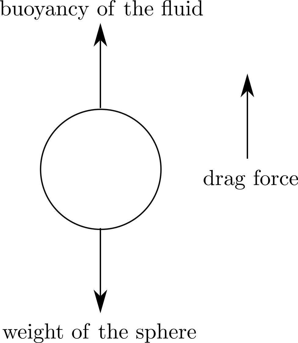
Balancing the forces on a steady fall we have
| (9.95) |
where
-
1.
no inertia (steady fall, no acceleration)
-
2.
weight of the sphere, density
-
3.
buoyancy (weight of displaced fluid, density )
-
4.
Stokes drag
E.g. For a ball bearing with density we can calculate the sedimenting speed for different fluids:
| Water: | ||||||
|---|---|---|---|---|---|---|
| Golden syrup: | 60 |
This experiment can be used to calculate the viscosity of different fluids.
Far-field approximation: Far away from the sphere, we can show that the disturbance looks like a point force. The velocity field when is
| (9.96) |
The force exerted across ‘’ must balance the force exerted across so the strength of the point force . Substituting this into the velocity field gives
| (9.97) |
This disturbance flow only knows the total force exerted and is independent of particle radius .