4A10 Flow instability Fluid-structure interaction CUED IIB Lecture notes 4 Galloping and flutter 6 Conduits and channels

Chapter 5 Vortex induced vibrations

The instability of galloping and flutter excite the natural mode of vibration of the structure in a situation where the fluid dynamic time scale is well-separated from the motion of the structure. The two scales are not so separated in the case of vortex induced vibrations. Underlying the vortex-induced vibrations is the purely fluid-dynamical instability of vortex shedding.

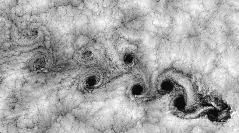
Refer to caption — Figure 5.1: von Karman vortex street generated as wind flows past the Juan Fernandez island, which is visualized in satellite imagery by passing clouds.

Any cylindrical bluff body immersed in a steady uniform flow sheds vortices alternating between each side of the body. Successive vortices are shed from alternating sides, even if the body cross section shape is symmetric. The vortex shedding has a well-defined frequency when the body is held stationary. These vortices are carried downstream and form the well-known von Karman vortex street. This phenomenon of vortex shedding is quite generic and is observed from the milimeter to the geological scales. For example, the vortex shedding past an island in the Pacific ocean is shown in fig. 5.1.

This causes a lift force of alternating sign on the body, which in turn causes the body to oscillate. The oscillations are naturally pronounced when the natural frequency of the structure that supports the body matches the naturally frequency of vortex shedding. Remarkably, if the natural structural frequency differs from the natural vortex shedding frequency, the process of vortex shedding alters itself so that vortices are shed at the natural frequency of the structure. These features of the phenomenon are the topic of this chapter.

5.1 Fluid dynamical instability

Consider a two-dimensional cross section shape, which is symmetric about the $x$ -axis, with a characteristic length $D$ . As an example, we will use the circular cross section with diameter $D$ . This shape is subject to a uniform flow of speed $U$ . The fluid is incompressible, has viscosity $\mu$ and density $\rho$ .

Figure 5.2: Schematic of the setup for analyzing vortex shedding.

The state variable is the Eulerian velocity field $\bm{u}(\bm{x},t)$ , which obeys the incompressible Navier-Stokes equations

\displaystyle\rho\left({\dfrac{\partial{\bm{u}}}{\partial{t}}}+(\bm{u}\cdot\bm% {\nabla})\bm{u}\right)=-\bm{\nabla}p+\mu\nabla^{2}\bm{u},\quad\text{and}\quad% \bm{\nabla}\cdot\bm{u}=0.

(5.1)

The variables are non-dimensionalized as presented in section 3.1 resultin in the dimensionless equations eq. 3.2 reproduced here as

\displaystyle{\dfrac{\partial{\bm{u}}}{\partial{t}}}+(\bm{u}\cdot\bm{\nabla})% \bm{u}=-\bm{\nabla}p+\dfrac{1}{\text{Re}}\nabla^{2}\bm{u},\quad\text{and}\quad% \bm{\nabla}\cdot\bm{u}=0,

(5.2)

where we have dropped the tilde decoration on the dimensionless variables for convenience, and chosen $L=D$ for the length scale and $T=D/U$ for the time scale. These are partial differential equations for the components $\bm{u}=(u,v)$ , which must be supplemented with appropriate boundary conditions. These are


$\displaystyle\bm{u}$	$\displaystyle=\bm{0},\quad\text{on the surface of the circle},$	(5.3a)
$\displaystyle\bm{u}$	$\displaystyle=\hat{\bm{e}}_{x},\quad\text{as }\|\bm{x}\|\to\infty.$	(5.3b)

Since no analytical solution to these equations with these boundary conditions is known, we must now proceed computationally. The solutions presented here are found using the commercial software COMSOL.

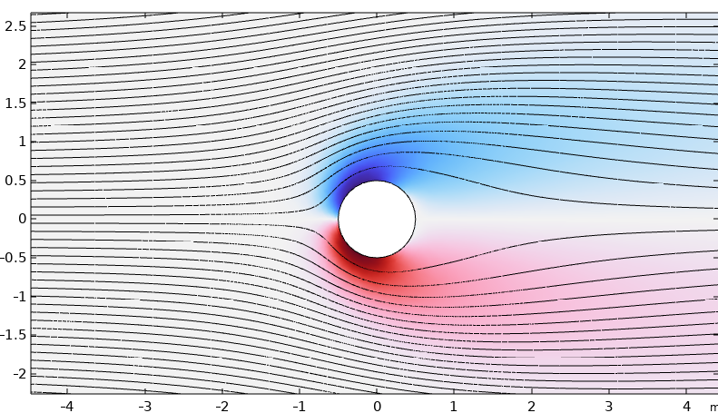
Here are the steps in the linear stability analysis. For each Reynolds number in a range, the steady state $\bm{u}=\bm{u}_{0}(\bm{x};\text{Re})$ is first calculated. An example is shown in fig. 5.3. The state is then perturbed as $\bm{u}=\bm{u}_{0}+\bm{u}^{\prime}$ , and the governing equations for $\bm{u}^{\prime}$ linearized as

\displaystyle{\dfrac{\partial{\bm{u}^{\prime}}}{\partial{t}}}+(\bm{u}_{0}\cdot% \bm{\nabla})\bm{u}^{\prime}+(\bm{u}^{\prime}\cdot\bm{\nabla})\bm{u}_{0}=-\bm{% \nabla}p^{\prime}+\dfrac{1}{\text{Re}}\nabla^{2}\bm{u}^{\prime},\quad\text{and% }\quad\bm{\nabla}\cdot\bm{u}^{\prime}=0,

(5.4)

where $p^{\prime}$ is the corresponding perturbation in pressure. Here we have used our judgment to non-dimensionalize the variables earlier in the process, so that step is not necessary any more. Hence we proceed to the next step of determining the eigenvalue problem by substituting $\bm{u}^{\prime}=\hat{\bm{u}}e^{st}$ , so that the mode shape $\hat{\bm{u}}$ and growth rate $s$ satisfies

\displaystyle s\hat{\bm{u}}+(\bm{u}_{0}\cdot\bm{\nabla})\hat{\bm{u}}+(\hat{\bm% {u}}\cdot\bm{\nabla})\bm{u}_{0}=-\bm{\nabla}\hat{p}+\dfrac{1}{\text{Re}}\nabla% ^{2}\hat{\bm{u}},\quad\text{and}\quad\bm{\nabla}\cdot\hat{\bm{u}}=0,

(5.5)

where $\hat{p}=p^{\prime}e^{-st}$ is the variable corresponding to pressure. There is a distinct possibility that the instability is oscillatory, so $\hat{\bm{u}}$ , $\hat{p}$ and $s$ are taken to be complex numbers.

The solution of the eigenvalue problem in eq. 5.5 is outside the scope of this document. (A sample will be shared in class from Zebib (1987)[10].)

All eigenvalues have a negative real part for $\text{Re}<\text{Re}_{c}\approx 47$ , where $\text{Re}_{c}$ is the critical Reynolds number. When the Reynolds number equals the critical value, the real part of two eigenvalues vanishe, while that of all the others remain negative. When the Reynolds number exceeds the critical, the real parts of those two eigenvalues are positive and signals exponential growth of the corresponding mode shape. Here two modes simultaneously become unstable because eigenvalues and eigenvectors must appear in complex conjugate pairs, so that the real perturbation that grows may be written as

\displaystyle\bm{u}^{\prime}=c_{1}\hat{\bm{u}}e^{st}+c_{1}^{*}\hat{\bm{u}}^{*}% e^{s^{*}t},

(5.6)

where superscript $*$ denotes complex conjugation.

The imaginary part of the eigenvalue, $\omega=\Im(s)$ , then gives the frequency of oscillations of the flow perturbation, which grows. This is, therefore, related to the (dimensional) frequency, $f$ , of vortex shedding of the growing perturbation as $f=\omega U/2\pi D$ . The frequency of vortex shedding is usually represented by the Strouhal number, $\text{St}=fD/U$ , which is then related to $\omega$ as $\text{St}=\omega/2\pi$ . Just as $\text{Re}_{c}$ is independent of the size of the cylinder or the nature of the fluid, St also represents the shedding frequency in a scale-independent manner. According to linear stability analysis, the St at the critical Re is around 0.1. However, the dynamics changes as the perturbation grows and reaches a finite amplitude, when it starts growing. In that state, the vortex shedding frequency is characterized by $\text{St}\approx 0.2$ . Experimentally measured Strouhal numbers as a function of Reynolds number for different shapes from page 50 of the book by Blevins[1] is shared separately in a handout.

The last piece of the puzzle is lift force on the cylinder. This is now an oscillating quantity with the same frequency as the vortex shedding and an amplitude that in a dimensionless form potentially depends on the Reynolds number and the object shape. This dependence is expressed as the lift coefficient as a function of Reynolds number, for example on page 64 of Blevins[1].

So far we have summarized the nature of the fluid dynamical instability that underlies vortex shedding around stationary cylinders. If the cylinders are mobile, we can now attempt to describe their response.

5.2 Vortex-induced vibrations

The basic idea is to model the cylinder as a one-dimensional structure with a mass, spring and damper, which is forced at the vortex shedding frequency in the direction of lift. If the displacement of the cylinder is $y$ , then following the notation of eq. 2.1, $y$ satisfies

\displaystyle m\ddot{y}+b\dot{y}+ky=F_{L}\sin\omega t,

(5.7)

where $F_{L}$ is the amplitude of the lift force and $\omega$ is the (dimensional) frequency.

Question 5.1.

Determine the steady periodic $y(t)$ satisfying eq. 5.7 and the amplitude of $y(t)$ .

Answer 5.1.

We start with non-dimensionalization, identical to that presented in eqs. 2.1 and 2.3, to get

\displaystyle\ddot{y}+2\beta\dot{y}+y=\sin{\Omega}t,

(5.8)

where we have dropped the tilde decoration and defined the non-dimensionalization of $y$ in terms of $F_{L}/k$ , and $\Omega=\omega/\omega_{0}$ . (The reader is reminded that $y$ was not non-dimensionalized in eq. 2.3.)

The solution is

\displaystyle y(t)=a\sin(\Omega t-\phi),\quad\text{where}\quad a=\left[(1-% \Omega^{2})^{2}+(2\beta\Omega)^{2}\right]\quad\text{and}\quad\tan\phi=\dfrac{2% \beta\Omega}{1-\Omega^{2}}.

(5.9)

Re-dimensionalizing the solution in eq. 5.9 is now a routine matter to predict the vortex-induced vibrations. This task is left to the industrious reader.

5.3 Mode locking

Due to this is a remarkable feature of vortex-induced vibrations, called mode locking, the structure can modify the vortex shedding frequency to a small extent. Suppose the (dimensional) natural frequency of the structure is $\omega_{0}$ and the natural vortex shedding frequency is $\omega_{f}$ , which are close to each other. Then the fluid dynamical vortex shedding instability is altered by the possible motion of the structure so that the joint vortex-induced vibrations frequency is $\omega_{0}$ .

5.4 Response to vortex shed by identical neighbours

Special care must be taken when designing identical structures that are susceptible to vortex-induced vibrations near each other, especially when no mechanism for damping is included. This is so because vortices shed that are shed from one structure apply an oscillating force on the second structure,so if the second is exactly downstream of the first when vortex-induced vibrations commence, the second become vulnerable to an additional forcing from the vortices of the first.

The following question illustrates this point.

Question 5.2.

Two poles 20 m tall and 0.2 m in diameter are erected 30 cm apart. Each pole is cantilevered to ground and free at the top. The pole is essentially a 1 cm thick pipe made of steel (density 7850 kg/m³ and Young’s modulus 200 GPa). Wind blows in a direction such that the wake of first pole is incident on the second, causing an oscillating lift force on the second. The second pole itself sheds vortices. The combined effect of the two processes is that the net amplitude of the oscillating lift on the second pole may be taken to be $C_{L}=1.3$ .

1.

Determine the natural frequency of the fundamental mode of oscillations of the tower.
2.

Let us take the Strouhal number for vortex shedding to be 0.2. Determine the wind speed for which the shedding frequency matches with the structural frequency of the fundamental mode.
3.

Assume the wind speed is according to the value found in the previous part. The drag coefficient for a cylinder is 0.7. Calculate the steady deflection of the pole. Ignore variation of the drag along the length of the pole.
4.

Assuming that the pole could still be considered to be straight, write the equation for the amplitude, $a(t)$ , of the fundamental mode of oscillation forced by the alternating lift force. Again, assume that the lift does not vary with length.
5.

Solve this equation and determine the amplitude of the tip of the pole.

Answer 5.2.

We answer in parts.

1.

Based on the geometry, the second moment of the cross section, $I$ is

$\displaystyle I=\pi(R_{o}^{4}-R_{i}^{4})=1.08\times 10^{-4}\textrm{ m}^{4},$

where $R_{o}$ and $R_{i}$ are the outer and inner radii of the tower. Based on this, the bending rigidity of the tower $B=EI$ is

$\displaystyle B=EI=2.16\times 10^{7}\textrm{ N~{}m}^{2},$

where $E$ is the Youngs modulus. Using the density of steel, $\rho$ , the mass per unit length, $\mu$ of the tower is

$\displaystyle\mu=\rho\pi(R_{o}^{2}-R_{i}^{2})=46.9\textrm{ kg/m}.$

Hence, from eq. 2.56, the natural frequency $\Omega_{1}$ of the fundamental mode is

$\displaystyle\Omega_{1}=k_{1}^{2}\sqrt{\dfrac{B}{\mu L^{4}}}=37\textrm{ rad/s}% ,\quad f_{1}=\dfrac{\Omega_{1}}{2\pi}=6\textrm{ Hz},$

where $f_{1}$ is the freuqncy.
2.

Using the definition of the Strouhal number and its value of 0.2

$\displaystyle U=\dfrac{f_{1}D}{\text{St}}=6\textrm{ m/s}\approx 20\textrm{ km/% h}.$
3.

Let $\rho_{a}$ be the density of air. The steady force on the pole per unit length is

$\displaystyle f_{D}=\dfrac{1}{2}\rho_{a}U^{2}(2R_{o})C_{D}=3\textrm{ N/m}.$

The tip deflection, $\delta$ , is

$\displaystyle\delta=\dfrac{f_{D}L^{4}}{8B}=2.7\textrm{ mm}.$
4.

The deflection of the beam satisfies

$\displaystyle\mu{\dfrac{\partial{{}^{2}h}}{\partial{t^{2}}}}+B{\dfrac{\partial% {{}^{4}h}}{\partial{x^{4}}}}=-\dfrac{1}{2}\rho_{a}U(2R_{o})C_{D}{\dfrac{% \partial{h}}{\partial{t}}}+\dfrac{1}{2}\rho_{a}U^{2}(2R_{o})C_{L}\sin\Omega_{1% }t.$

In this equation, the term proportional to $C_{D}$ is determined from considerations identical to eq. 4.6. A moments inspection will immediately convince the reader that the term proportional to $C_{D}$ act as a damping and is relatively quite weak compared to either the inertial term or the bending term for the fundamental mode of vibrations. Yet it is important to retain this term. Multiplying by the mode shape, $y_{1}(x/L)$ from eq. 2.57, and integrating gives the equation for the amplitude of fundamental mode as

$\displaystyle\ddot{a}+2\beta\dot{a}+\Omega_{1}^{2}a=f_{L}\sin\Omega_{1}t,$

where

$\displaystyle f_{L}=\dfrac{1}{2}\dfrac{\rho_{a}U^{2}(2R_{o})C_{L}}{\mu}\left(% \dfrac{\int_{0}^{1}y_{1}(s)~{}\textrm{d}s}{\int_{0}^{1}y_{1}^{2}(s)~{}\textrm{% d}s}\right)\approx 0.10\textrm{ m/s}^{2}\quad\text{and}\quad\beta=\dfrac{1}{4}% \dfrac{\rho_{a}U(2R_{o})C_{D}}{\mu}\approx 5.3\times 10^{-3}\textrm{ s}^{-1}.$

Here, the mode shape is scaled such that $y_{1}(1)=1$ , so that the deflection of the tip is unity.
5.

The solution proceeds along the lines similar to question 5.1 but is simplified because the forcing frequency is equal to the natural frequency. In this case the solution is

$\displaystyle a(t)=-a_{0}\cos\Omega_{1}t\quad\text{where}\quad a_{0}=\dfrac{f_% {L}}{2\beta\Omega_{1}}\approx 25.7\text{ cm!}$

The amplitude of the vortex-induced vibrations is nearly a 100 times bigger than the static deflection of the pole under the wrong wind conditions.

Note that in question 5.2, the dominant damping of the vibrations comes from the fluid itself. The metal itself provides extremely small amount of damping, which is why tuning forks vibrate for as long as they do. Radiation of sound from the vibrations is another source of damping, the dominant one for the tuning fork, but for the pole sound radiation is negligible compared to the damping due to the drag.

Finally, note that for a single pole, vortex-shedding applies a lift force with $C_{L}\approx 0.2$ , so that the deflection of the upstream pole would be smaller by a factor $1.3/0.2\approx 6.5$ . But it is the vortices shed by the upstream pole that causes and much larger oscillating force on the downstream one. If these structures are designed merely to sustain their own vortex shedding force, without accounting for the vortices shed from the other pole, they would almost certainly fail when the wind aligns.

5.5 Suppressing vortex-induced vibrations

Mechanisms to suppress vortex-induced vibrations fall in the following categories:

1.

Avoiding resonance by stiffening the structure. This intervention is obvious to avoid large amplitude oscillations.
2.

Streamline the cross section. Doing so reduces the possibility of alternate vortices shed and also reduces their strength by diminishing their magnitude. It may not always be possible to change the cross section.
3.

Add vortex suppression device. These devices disrupt the synchrony of the vortex-shedding process. Examples include helical strakes, perforated shrouds, axial slats, etc. These examples and more are shown in Figure 3-23 on page 78 of the book by Blevins[1].
4.

Add or increase damping. This method is not always possible or may be too expensive. Dampers may be passive, such as a dashpot, or active, such as the tuned-mass damper. An entertaining account is presented in this popular video.

5.6 Conclusion

Vortex-induced vibrations are an example of a flow instability that drives a structure. This is unlike the other examples we have seen, such as galloping and flutter. In all these example, the natural modes of oscillation are excited by a fluid flow, whether or not the flow adjusts quasisteadily to the instantaneous geometry of the structure. We have presented the outline of the purely fluid dynamical instability in section 5.1 and then the forcing of the structural mode in section 5.2. However, this treatment is approximate because the in the fluid dynamical stability analysis, the no-slip boundary condition was imposed on the surface of the stationary cylinder. In vortex-induced vibrations, the cylinder is not stationary. Thus, our analysis is necessarily approximate. The exact linear stability analysis with the moving cylinder is outside the scope of this document.